how a neuron learns

warning: this is an extremely simplified explanation. if you want to delve deeper, there are excellent resources like Andrew Ng’s Deep Learning Specialization or Neural Networks from Scratch in Python.

this is a neural network. you’ve likely seen one before and have, at least, a vague idea of what it does : it learns. what you may not know is that they can be thought of as universal function approximators. that might seems abstract to you, so let’s look at the definition of a function

In mathematics, a function from a set \(X\) to a set \(Y\) assigns to each element of \(X\) exactly one element of \(Y\). The set \(X\) is called the domain of the function and the set \(Y\) is called the codomain of the function.

if this seems too theoretical, imagine a function as a black box that takes an input \(x\) and returns an output \(y\). this concept is powerful, as almost anything can be represented as a function. for example, reading this post involves processing pixel input and outputs an understanding of words. theoretically, a sufficiently large neural network could replicate this process.

but how is it able to do that? well, to understand this, let’s examine a single layer

we start with inputs, \({x_1, x_2, ..., x_n} \in X\), which could be from the input layer, like the pixels of an image, or from a previous layer in the network. then we have neurons, or perceptrons, symbolized by \(\Sigma\). perceptrons, the basic unit of a neural network, assign a weight to every input. each weight is multiplied by its corresponding input and then summed. for each input layer, there’s an input of 1, allowing each perceptron to create a bias. think of this as a constant (the \(b\) in \(y = mx + b\)).

this means perceptrons build multivariate linear functions. from inputs \({x_1, x_2, ..., x_n}\), a perceptron outputs \(z = w_1 \cdot x_1 + w_2 \cdot x_2 + ... + w_n \cdot x_n + b\).

the output \({z_1, z_2, z_n }\) of a layer then goes through an activation function \(\phi\) which introduces non-linearity, we will study the importance of this in another post.

we see that a single layer can approximate multivariate functions. but how does a perceptron learn a specific function? let’s begin with the simplest example: a single perceptron with one input.

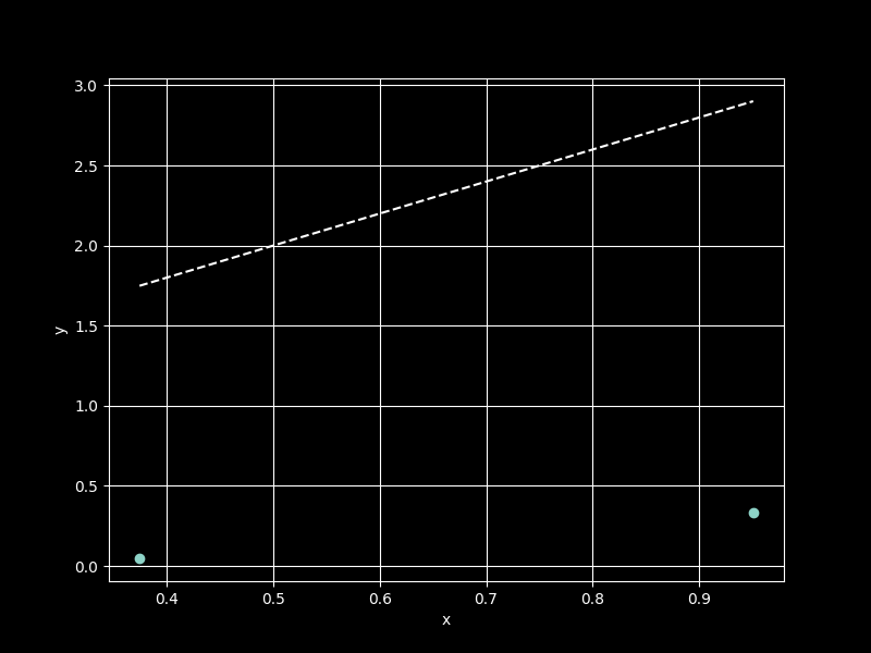
now, let’s construct the function \(y = 2x + 1\). a linear function can be represented by two points, so let’s plot them in python:

import numpy as np
import matplotlib.pyplot as plt

# Generating input values
np.random.seed(42)
x_values = np.random.rand(2, 1)

# Calculating true values of the function
y_values = 2 * x_values + 1

plt.figure(figsize=(8, 6))
plt.scatter(x_values, y_values, label='True function: 2x + 1')
plt.xlabel('x')
plt.ylabel('y')
plt.grid(True)
plt.show()

we now have two input-output pair to feed to our perceptron, [[0.37454012][0.95071431]] and [[1.74908024][2.90142861]]. the perceptron needs to adjust its weight to 2 and its bias to 1 using only this data.

let’s initialize it with random values.

np.random.seed(42)
w = np.random.randn()
b = np.random.randn()

print(f"Weight: {w:.4f}, Bias: {b:.4f}")

def forward(x):
    return w * x + b

y_hat_values = [forward(x) for x in x_values]

Weight: 0.4967, Bias: -0.1383

unsurprisingly, the perceptron’s \(\hat{y}\) values did not succeed in approximating the function on the first try. therefore, we need to quantify how much the model’s predictions differ from the actual values and determine the influence of the weight and bias parameters on the error in order to correct them. for this purpose, we use a loss function (or cost function) that will

1. quantify the error in prediction with respect to the weight and bias
2. have its value lower as the prediction improves

for regression problems, like function approximation, the Mean Squared Error (MSE) is often used.

the MSE is defined as follows, where n is the number of training examples, \(y_i\) is the actual values, and \(\hat{y}_i\) is the model’s predictions: \(MSE = \frac{1}{n} \sum_{i=1}^{n} (y_i - \hat{y}_i)^2\)

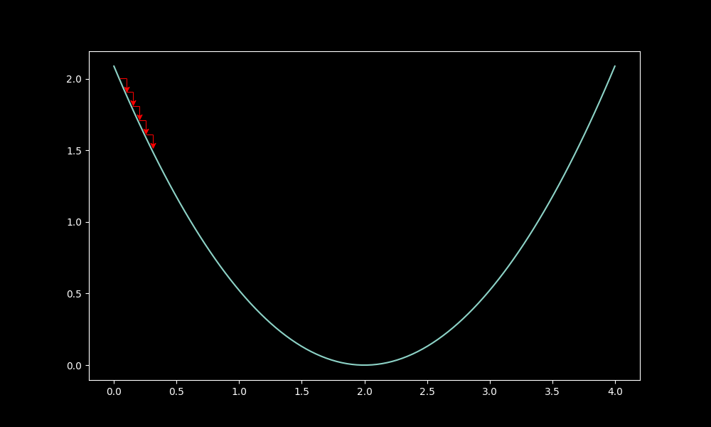
to simplify the calculations, our cost function will be defined as \(\mathcal{C} = \frac{MSE}{2}\). to understand this choice of cost function, we can visualize it:

in particular, with respect to the weight parameter:

this function is ideal for minimizing error relative to the parameters. by analyzing the gradient, which shows the direction of increasing loss, we minimize the loss by moving in the opposite direction. this is basis of the gradient descent algorithm.

we calculate gradients using the chain rule:

and

given that \(\mathcal{C}= \frac{1}{2n} \sum_{i=1}^{n} (y_i - \hat{y}_i)^2\) and \(\hat{y}=wx+b\) with \(x\) as the input, we have:

and

here, n=2 with \(x_1, x_2\) being the inputs or x_values, \(y_1, y_2\) being the outputs of the function \(f : x \mapsto 2 \cdot x + 1\) or y_values and \(\hat{y}_1, \hat{y}_2\) being the outputs of the perceptron for x_values, or y_hat_values

after calculating the gradient, we update the parameters using a learning rate (lr), typically between 0.001 and 0.1. the updating formula is:

w -= gradient(w) * lr

b -= gradient(b) * lr

this is called a step, adjusting the parameters to minimize the loss. the learning rate shouldn’t be too small to avoid excessive steps

nor too high, as it may worsen the loss:

in this example, each step will be done after having measured the loss for the full epoch, which is a complete training phase where the neural network sees the entire training dataset (in our case, two points) once.

now, let’s build our entire training pipeline:

np.random.seed(42)
x_values = np.random.rand(2, 1)
y_values = 2 * x_values + 1

w = np.random.randn() 
b = np.random.randn()  

lr = 0.1  # learning rate

def forward(x):
    return w * x + b

# cost function (MSE/2)
def criterion(y_true, y_hat):
    return 1/2 * np.mean((y_true - y_hat)**2)

num_epochs = 1001
losses = []

for epoch in range(num_epochs):
    y_hat = forward(x_values)

    loss = criterion(y_values, y_hat)
    losses.append(loss)

    dw = (1/len(x_values)) * np.sum((y_hat - y_values) * x_values)
    db = (1/len(x_values)) * np.sum(y_hat - y_values)

    # Updating parameters
    w -= lr * dw
    b -= lr * db

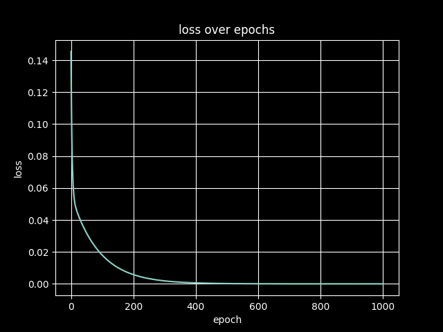
    if epoch % 100 == 0:
        print(f'epoch {epoch}, loss: {loss:.4f}')
print("============================")
print(f"weight: {w:.4f}, bias: {b:.4f}"")
print("============================")

epoch 0, loss: 0.1455
epoch 100, loss: 0.0180
epoch 200, loss: 0.0058
epoch 300, loss: 0.0019
epoch 400, loss: 0.0006
epoch 500, loss: 0.0002
epoch 600, loss: 0.0001
epoch 700, loss: 0.0000
epoch 800, loss: 0.0000
epoch 900, loss: 0.0000
epoch 1000, loss: 0.0000
============================
weight: 1.9961, bias: 1.0027
============================

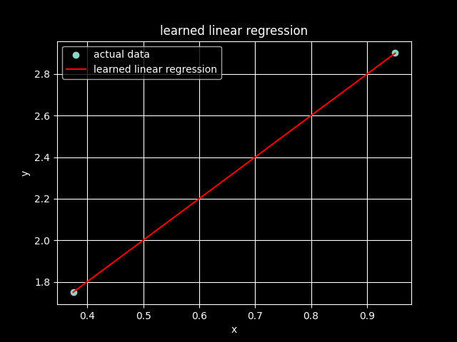
we observe that our perceptron successfully learned the parameters of our function using only the input and output data. we will study in another post how a network of perceptrons can learn more complex functions.